This past month, our development team successfully finished porting some of MATLAB’s basic numerical methods to the Multiprecision Computing Toolbox, enabling calculations in the arbitrary precision. At this point in time, the following routines for numerical integration, optimization, and ordinary differential equations are now available:
% Integration
quad	        % Numerically evaluate integral, adaptive Simpson quadrature
quadgl	        % Numerically evaluate integral, fixed Gauss-Legendre quadrature
dblquad	        % Numerically evaluate double integral over rectangle
triplequad	% Numerically evaluate triple integral

% Optimization
fminsearch	% Find minimum of unconstrained multivariable function (Nelder–Mead simplex search)
fzero	        % Find root of continuous function of one variable
optimset	% Create or edit optimization options structure
optimget	% Optimization options values

% Ordinary differential equations
ode45	        % Solve initial value problems for ordinary differential equations
odeget	        % Ordinary differential equation options parameters
odeset	        % Create or alter options structure for ordinary differential equation solvers
All new functions are fully compatible with MATLAB’s built-in analogs. In fact, most of the listed functions above are simply MATLAB’s codes ported to the multiprecision arithmetic with the aid of the Toolbox.
To demonstrate the improved optimization methods, we can find the global minimum of Rosenbrock’s banana function with 35 digits accuracy:
>> mp.Digits(40);
>> banana = @(x)100*(x(2)-x(1)^2)^2+(1-x(1))^2;
>> options = optimset('Display','iter','TolX',mp('1e-35'),'TolFun',mp('1e-35'));
>> [x,fval] = fminsearch(banana,mp([-1.2, 1]),options)          % True minimum is at (1,1)

Optimization terminated:
 the current x satisfies the termination criteria using OPTIONS.TolX of 1e-35
 and F(X) satisfies the convergence criteria using OPTIONS.TolFun of 1e-35

1.000000000000000000000000000000000001627    1.000000000000000000000000000000000003447

6.36301990841906554427230354356822760322e-72
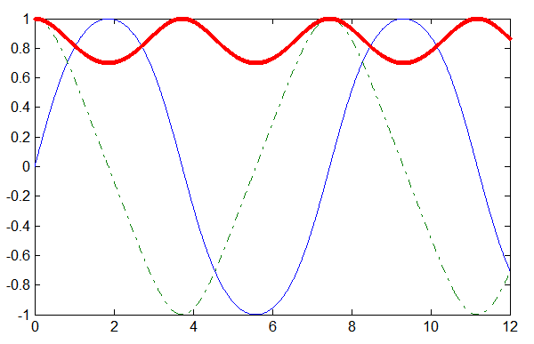
The following example illustrates the solution of a system of equations describing the motion of a rigid body without external forces (Example 1 in MATLAB documentation):
% System of ODE
function dy = rigid(t,y)
dy = zeros(3,1);    % a column vector
dy(1) = y(2) * y(3);
dy(2) = -y(1) * y(3);
dy(3) = -0.51 * y(1) * y(2);
end

% Solving with accuracy of 10 digits
options = odeset('RelTol',mp('1e-10'),'AbsTol',repmat(mp('1e-10'),1,3));
[T,Y] = ode45(@rigid,mp([0 12]),mp([0 1 1]),options);

plot(double(T),double(Y(:,1)),'-',double(T),double(Y(:,2)),'-.',double(T),double(Y(:,3)),'.')


{ 0 comments… add one now }